-
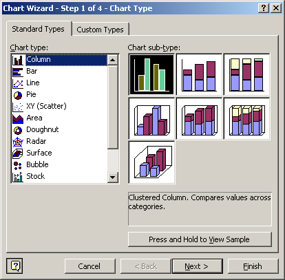
The Chart Wizard starts at Step 1 by asking what type of
chart to make (see screen shot ).
-
Select a chart type and sub-type that works
best for your data and click the Next button.
- At Step 2 of the Chart Wizard, observe if chart is displaying the data correctly. If not use the option buttons and list boxes at this step to adjust the chart data. If the chart appears OK, click the Next button.
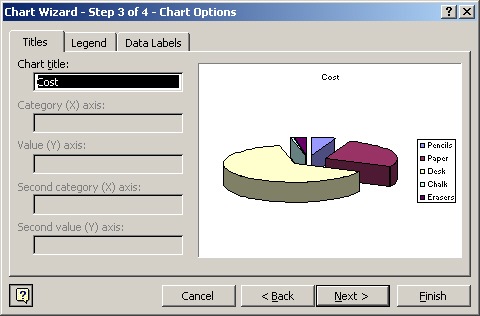
- At Step 3 of the Chart Wizard is where the chart's titles, legend, and data labels are controlled.
- Starting from the Titles tab, change the chart title if desired.
Note: It is sometimes a better choice to use labels instead of the legend if the chart is to be printed or photocopied, as distinctions in grayscale are hard to decipher.
- Click the Legend tab and clear the "Show Legend" checkbox.
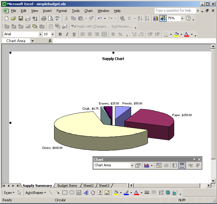
- Click the Data Labels tab and select both Category Name and Value for labels.
- If using a Pie Chart, clear the Show Leader Lines option because the pie sections are few and the labels should be clear without leader lines.
- Click the Next button to continue.